Free-energy surfaces from an ASE trajectory

MMML can estimate a one- or two-dimensional free-energy surface (FES) from scalar coordinates evaluated on an ASE trajectory. The estimator constructs a histogram and calculates

[ F(q) = -R T \ln P(q), ]

with the minimum occupied-bin energy shifted to zero. This is an empirical FES of the sampled trajectory; reliable barriers require equilibrated sampling and adequate transitions between metastable states.

Load a trajectory

from ase.io import read

frames = read("/Users/ericboittier/test4.pdb", index=":")
print(len(frames), "frames")
print(len(frames[0]), "atoms per frame")

test4.pdb contains 288 frames. Each frame has a capped peptide in a periodic water box. ASE uses zero-based atom indices. For this topology, the central backbone coordinates are:

• phi: C-N-CA-C, atoms (4, 6, 8, 14)
• psi: N-CA-C-N, atoms (6, 8, 14, 16)

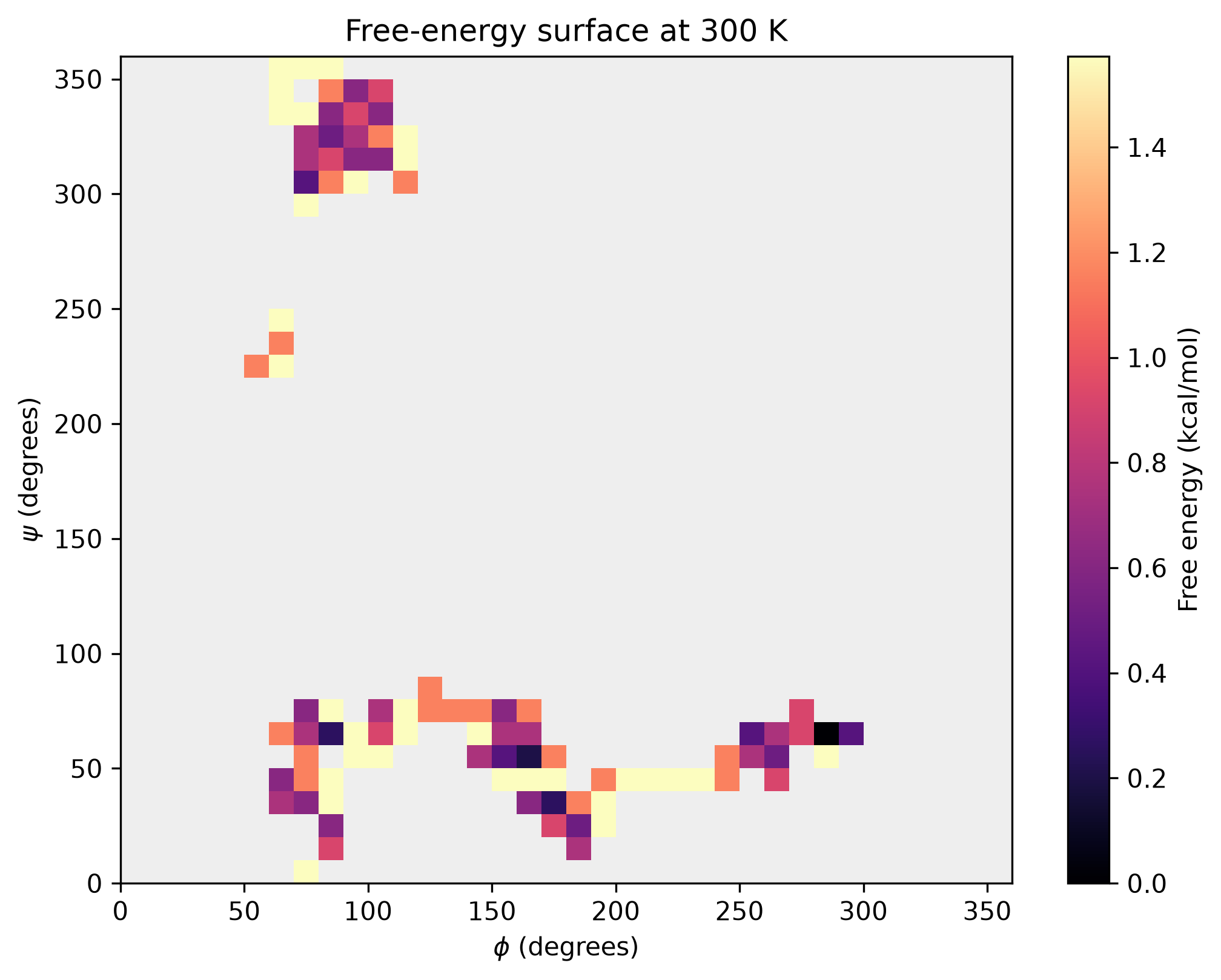
Calculate a two-dimensional phi/psi FES

ASE reports dihedrals in the interval 0–360 degrees. Coordinate functions can be arbitrary Python callables that accept one ase.Atoms frame and return one scalar.

from mmml.utils.plotting import fes_from_trajectory, plot_fes

phi = lambda atoms: atoms.get_dihedral(4, 6, 8, 14, mic=True)
psi = lambda atoms: atoms.get_dihedral(6, 8, 14, 16, mic=True)

phi_psi_fes = fes_from_trajectory(
    frames,
    [phi, psi],
    temperature_k=300.0,
    bins=(36, 36),
    ranges=((0.0, 360.0), (0.0, 360.0)),
    energy_unit="kcal/mol",
)

fig, ax = plot_fes(
    phi_psi_fes,
    labels=(r"$\phi$ (degrees)", r"$\psi$ (degrees)"),
    max_free_energy=5.0,
)

Calculate a one-dimensional profile

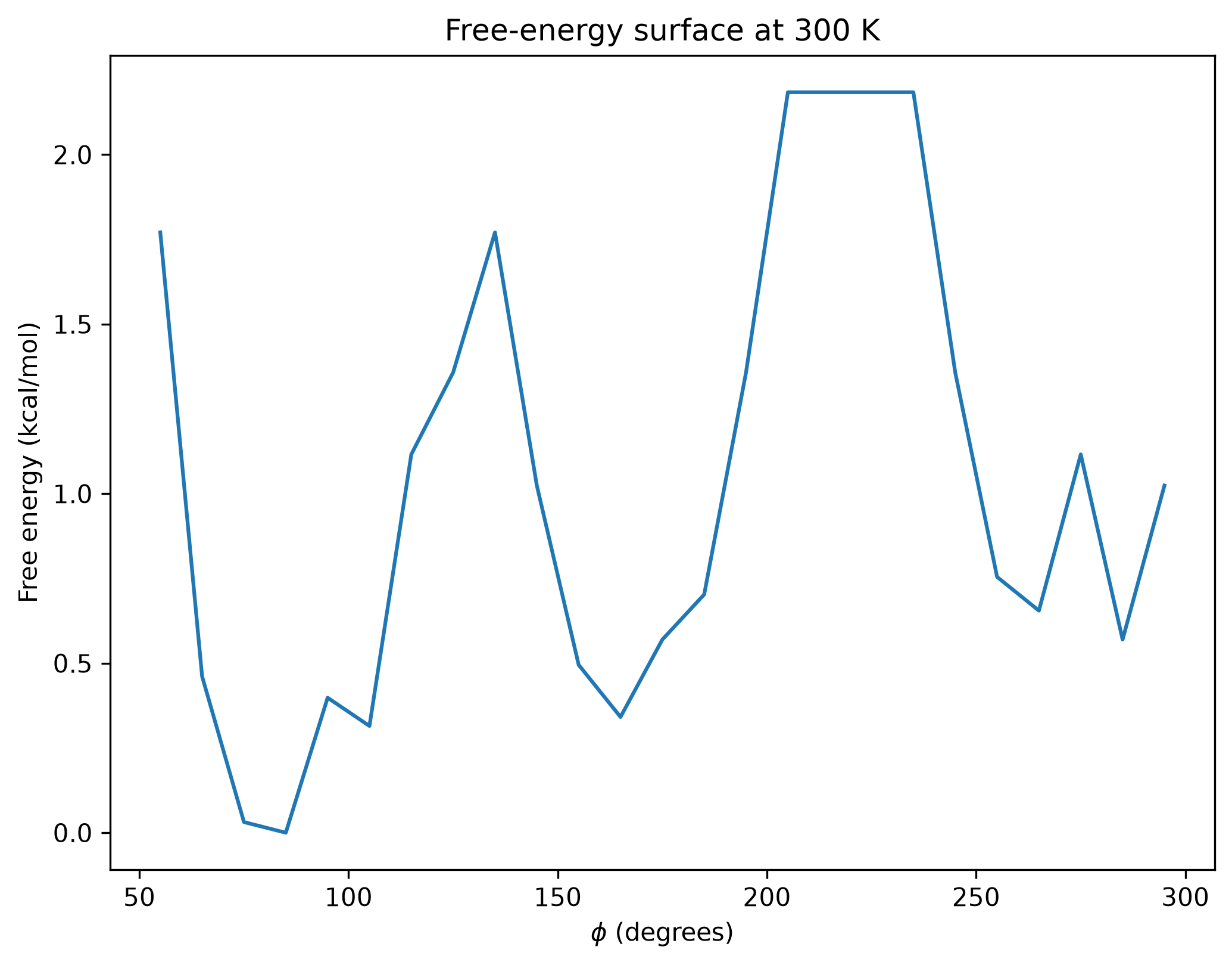
Pass one coordinate to obtain a free-energy profile.

phi_fes = fes_from_trajectory(
    frames,
    [phi],
    temperature_k=300.0,
    bins=36,
    ranges=((0.0, 360.0),),
)

fig, ax = plot_fes(
    phi_fes,
    labels=(r"$\phi$ (degrees)",),
    max_free_energy=5.0,
)

The same pattern works for any scalar coordinate, for example:

distance = lambda atoms: atoms.get_distance(0, 18, mic=True)
angle = lambda atoms: atoms.get_angle(4, 6, 8, mic=True)
radius_of_gyration = lambda atoms: atoms[:22].get_moments_of_inertia().sum()

For biased or reweighted trajectories, evaluate coordinates explicitly and pass one statistical weight per frame to calculate_fes:

from mmml.utils.plotting import calculate_fes, evaluate_coordinates

samples = evaluate_coordinates(frames, [phi, psi])
surface = calculate_fes(samples, weights=frame_weights, bins=(36, 36))

Empty histogram bins are assigned a finite display floor. They are not sampled free-energy estimates and should not be interpreted as physical barriers.

RDFs and internal degrees of freedom

The companion structural-analysis utilities operate directly on the same list of ASE frames:

from mmml.utils.plotting.trajectory_structure import (
    element_pair_rdfs,
    internal_coordinate_distributions,
)

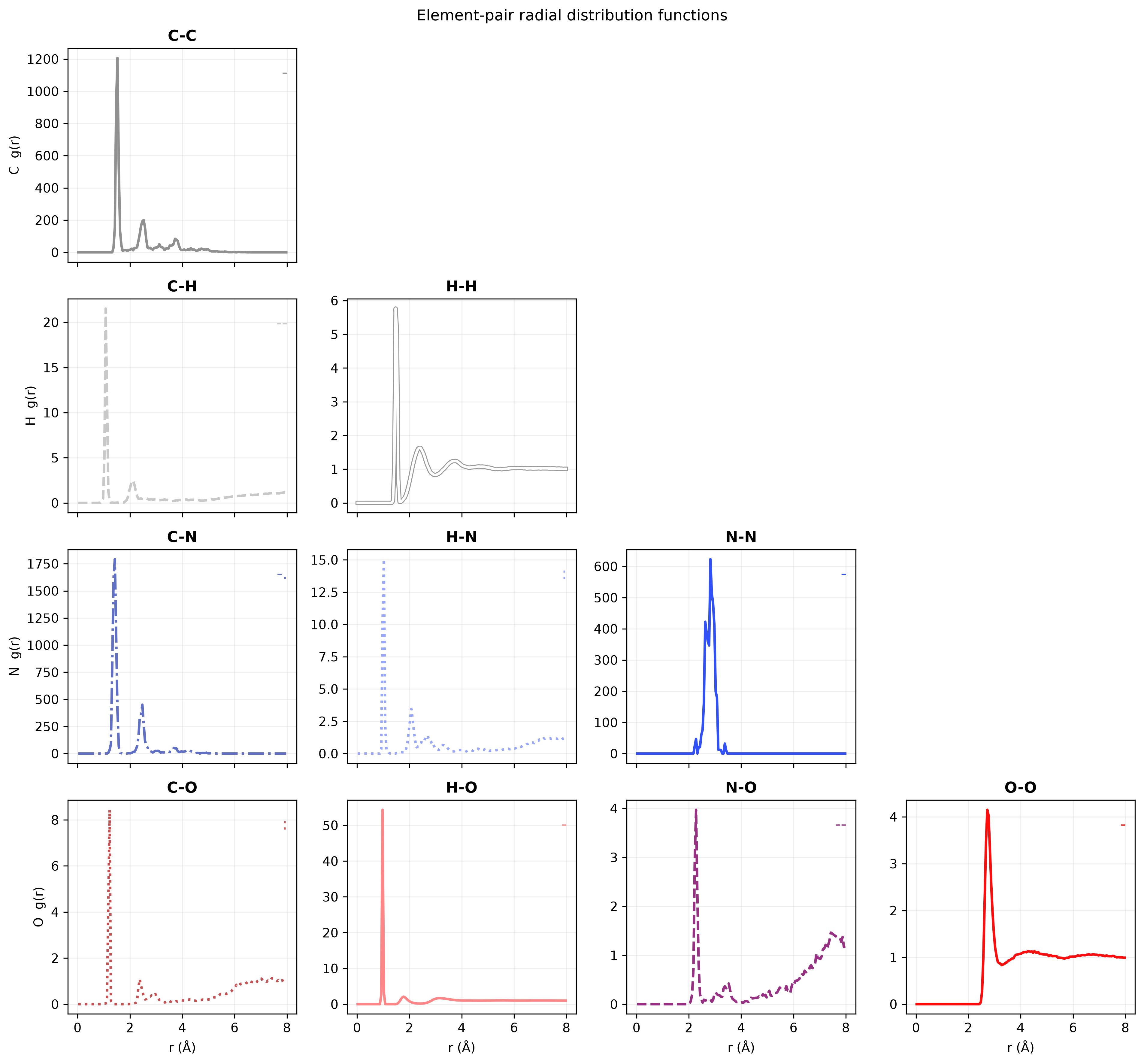
radii, rdfs = element_pair_rdfs(frames, r_max=8.0, bins=160)
internal = internal_coordinate_distributions(frames, range(22))

plt.plot(radii, rdfs["O-O"])
plt.xlabel("r (Å)")
plt.ylabel("g(r)")

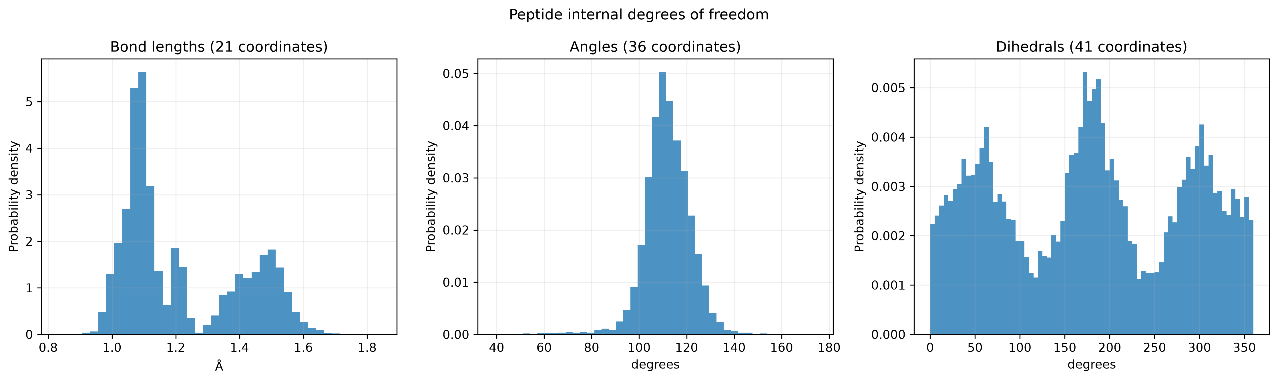
The RDF normalization uses the periodic cell volume and unique atom pairs. internal contains one trajectory array per inferred peptide bond, angle, and proper dihedral. Covalent connectivity is inferred from 1.2 times the tabulated covalent radii.

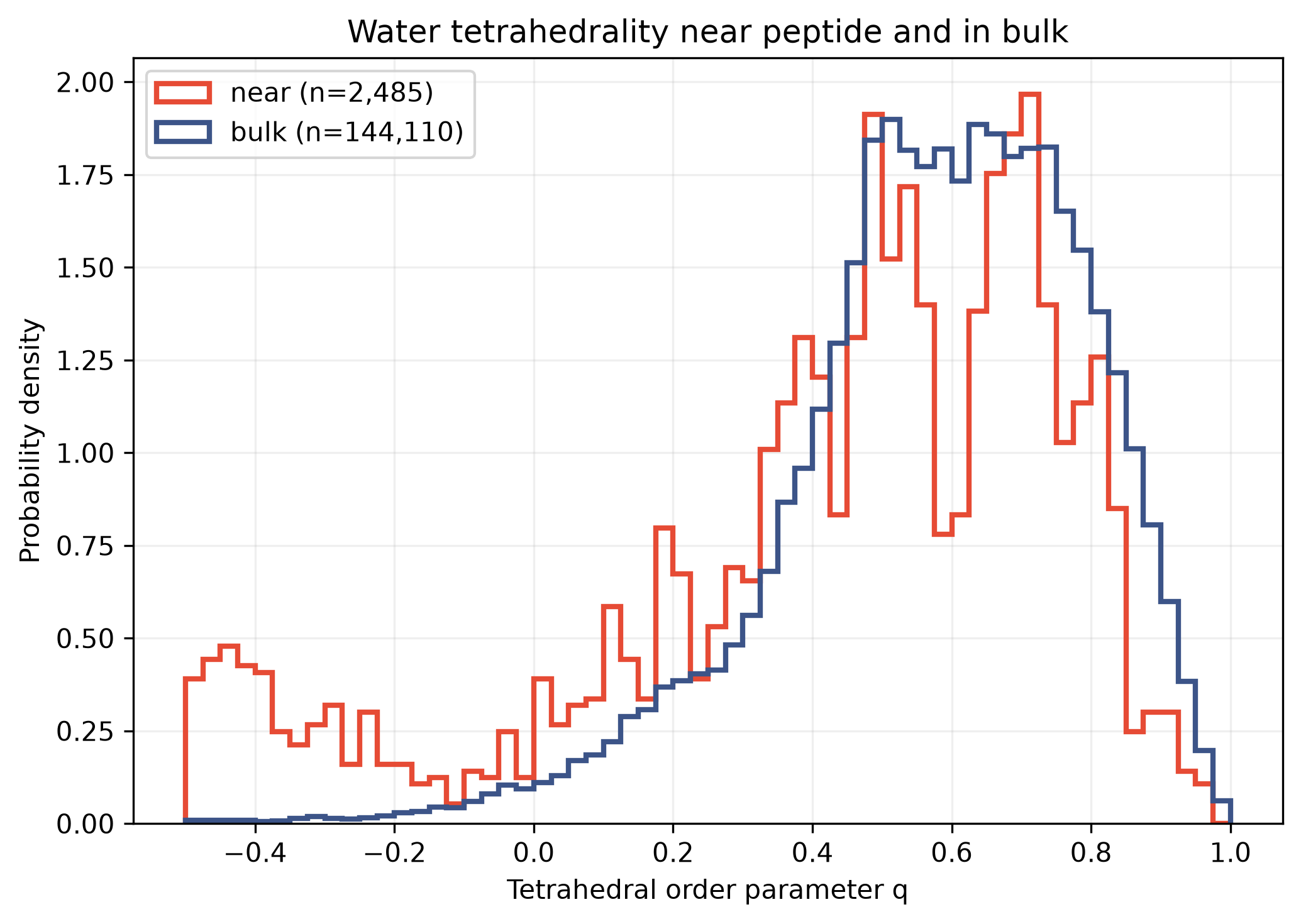
Water tetrahedrality

The tetrahedral order parameter is calculated from the four nearest oxygen neighbors of each water oxygen:

[ q = 1 - \frac{3}{8}\sum_{j<k}^{4} \left(\cos\psi_{jk} + \frac{1}{3}\right)^2. ]

For this example, a water is near the peptide when its oxygen is within 5 Å of any peptide heavy atom. A water is bulk-like when that minimum distance is at least 8 Å. Waters in the 5–8 Å transition region are omitted from this comparison. All distances and nearest-neighbor vectors use the periodic minimum-image convention.

from mmml.utils.plotting.trajectory_structure import water_tetrahedrality

tetrahedrality = water_tetrahedrality(
    frames,
    peptide_indices=range(22),
    near_cutoff=5.0,
    bulk_cutoff=8.0,
)

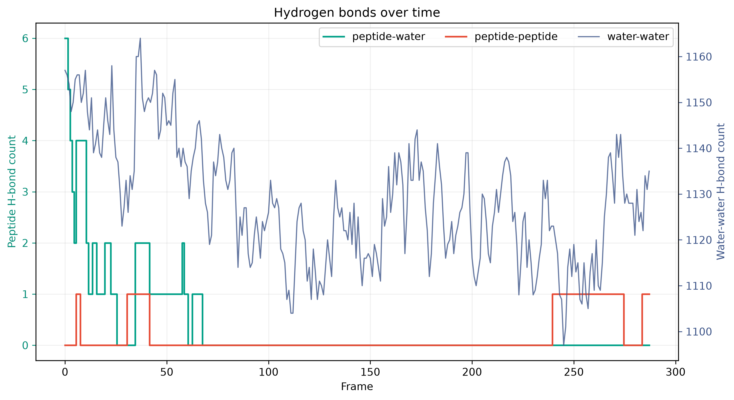
Hydrogen bonds and interaction network

Hydrogen bonds are detected with a deliberately permissive donor–acceptor distance no greater than 3.8 Å and a D–H···A angle of at least 135°. Nitrogen and oxygen atoms are treated as acceptors and as donors when covalently bound to hydrogen. Distances and angles use periodic minimum-image vectors.

from mmml.utils.plotting.trajectory_structure import hydrogen_bond_analysis

hydrogen_bonds = hydrogen_bond_analysis(
    frames,
    peptide_indices=range(22),
    distance_cutoff=3.8,
    angle_cutoff_degrees=135.0,
)

plt.plot(hydrogen_bonds.peptide_water_counts, label="peptide-water")
plt.plot(hydrogen_bonds.peptide_peptide_counts, label="peptide-peptide")
plt.legend()

The NetworkX diagram uses the frame with the largest total hydrogen-bond count. All atoms are shown at their wrapped Cartesian x/y coordinates with low opacity. Hydrogen-bond edges include the complete water–water network as well as peptide–water and peptide–peptide interactions. The edge colors and legend separate those three classes. Peptide atoms retain labels; water atom labels are suppressed to keep the dense network readable.

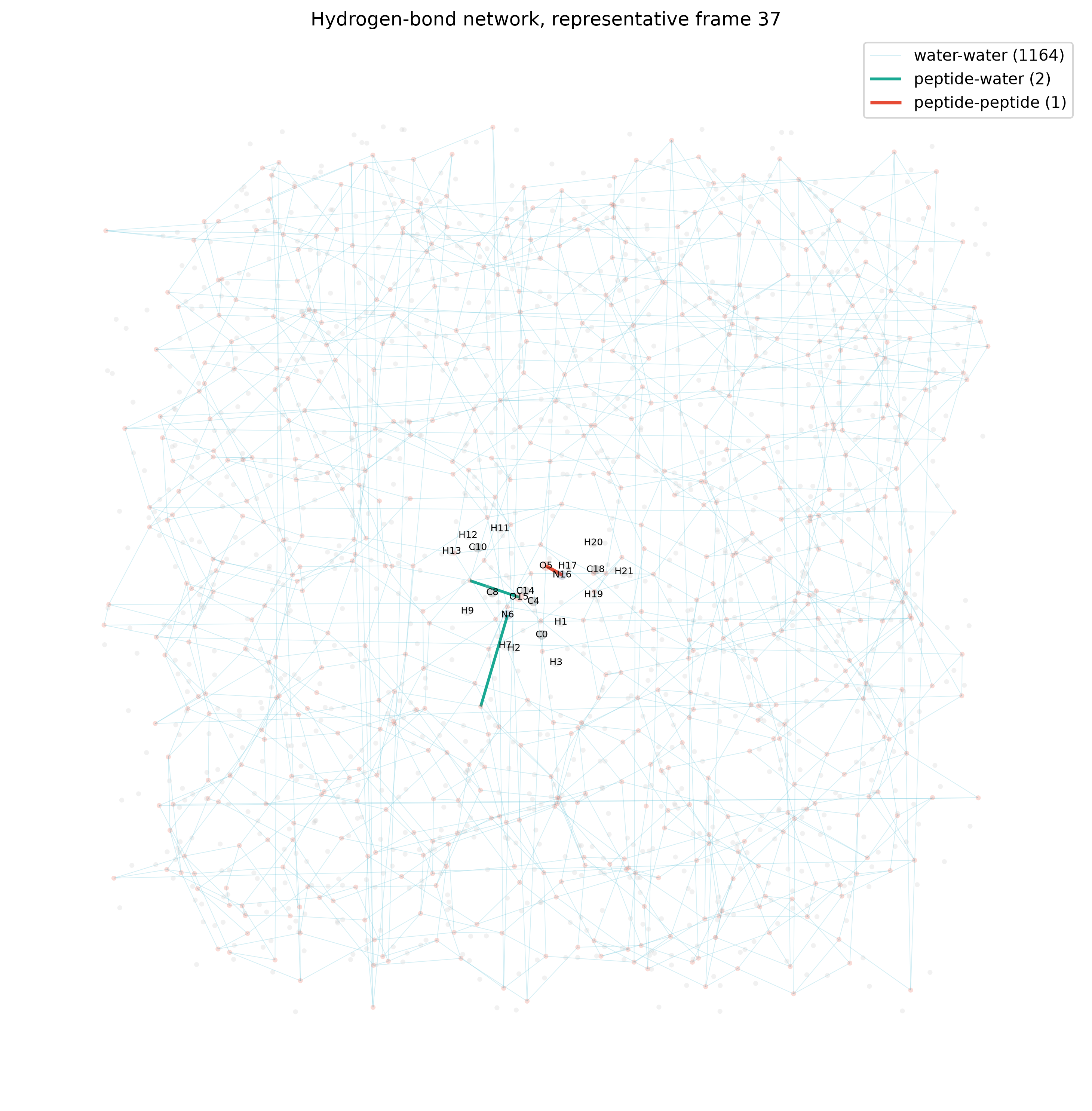
The corresponding arrays and edge occupancies are saved in test4_hydrogen_bonds.npz.

Radius of gyration, MSD, and diffusion

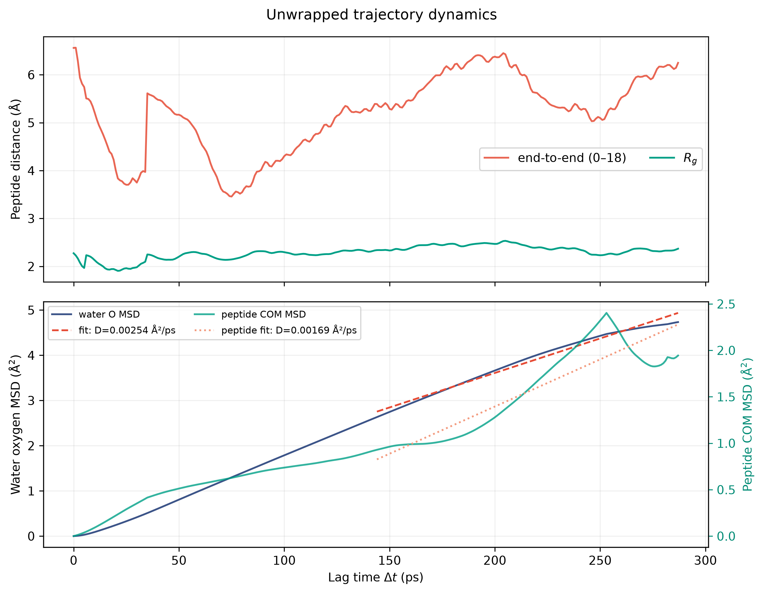
Wrapped coordinates must not be used directly for mean-squared displacement. MMML reconstructs continuous fractional coordinates from frame-to-frame minimum-image displacements and raises if a displacement reaches the half-cell ambiguity limit. The peptide radius of gyration is mass weighted and calculated from these unwrapped coordinates. End-to-end distance is the direct unwrapped Cartesian separation between configurable endpoint atoms; this example uses terminal heavy atoms 0 and 18. Water diffusion uses the ensemble MSD of all water oxygen atoms:

[ \mathrm{MSD}(t)=\left\langle|\mathbf r_i(t)-\mathbf r_i(0)|^2\right\rangle_i, \qquad D=\frac{1}{6}\frac{d\,\mathrm{MSD}}{dt}. ]

from mmml.utils.plotting.trajectory_structure import (
    radius_of_gyration_and_diffusion,
    unwrap_trajectory_positions,
)

unwrapped_positions = unwrap_trajectory_positions(frames)
dynamics = radius_of_gyration_and_diffusion(
    frames,
    peptide_indices=range(22),
    timestep_ps=1.0,
    fit_start_fraction=0.5,
    end_to_end_indices=(0, 18),
)
print(dynamics.diffusion_angstrom2_per_ps)

The PDB does not contain timing metadata. The generated example therefore uses 1 ps per saved frame only as an explicit placeholder. Replace timestep_ps=1.0 with the actual saved-frame interval before interpreting the diffusion coefficient. The fitted coefficient scales inversely with this value. The reported independent variable is lag time, (\Delta t), rather than absolute trajectory time. Both water and peptide center-of-mass MSDs average over every available time origin for each lag. The fit shown below uses the final 50% of lag times; production diffusion estimates should still verify the linear diffusive regime and assess fit-window sensitivity.

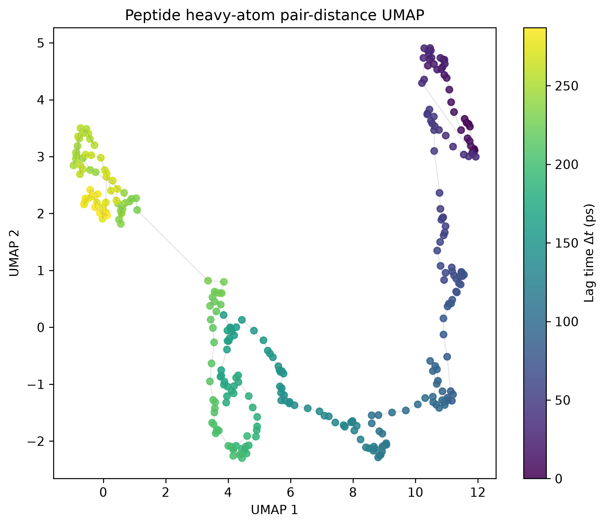
Heavy-atom distance UMAP

For conformational dimensionality reduction, raw Cartesian coordinates are a poor default because translations and rotations dominate their variance. Instead, MMML computes every pair distance among the peptide heavy atoms, standardizes each distance feature, and embeds the resulting frame-by-feature matrix with two-dimensional UMAP. For this peptide there are 10 heavy atoms and 45 pair-distance features.

from mmml.utils.plotting.trajectory_structure import heavy_atom_pair_distance_umap

embedding, pair_distances, heavy_atom_pairs = heavy_atom_pair_distance_umap(
    frames,
    peptide_indices=range(22),
    n_neighbors=20,
    min_dist=0.1,
    random_state=42,
)

Points are colored by lag from the first saved frame and connected in trajectory order. UMAP coordinates have no physical units; cluster separation is useful for exploring conformational states but should be checked against interpretable coordinates such as phi, psi, radius of gyration, and end-to-end distance.